MNIST with PyTorch

All tutorials in Jupyter Notebook format are available for download. You can either download them to a local computer and upload to the running Jupyter Notebook or run the following command from a Jupyter Notebook Terminal running in your Kaptain installation:

CODE

curl -L https://downloads.d2iq.com/kaptain/d2iq-tutorials-2.2.0.tar.gz | tar xz

These notebook tutorials have been built for and tested on D2iQ's Kaptain. Without the requisite Kubernetes operators and custom Docker images, these notebooks will likely not work.

Training MNIST with PyTorch

Introduction

Recognizing handwritten digits based on the MNIST (Modified National Institute of Standards and Technology) data set is the “Hello, World” example of machine learning. Each (anti-aliased) black-and-white image represents a digit from 0 to 9 and fits in a 28×28 pixel bounding box. The problem of recognizing digits from handwriting is, for instance, important to the postal service when automatically reading zip codes from envelopes.

What You Will Learn

You will see how to use PyTorch to build a model with two convolutional layers and two fully connected layers to perform the multi-class classification of images provided. In addition, there is a dropout layer after the convolutional layers (and before the first fully connected layer) and another one right after the first fully connected layer.

The example in the notebook includes both training a model in the notebook and running a distributed PyTorchJob on the cluster, so you can easily scale up your own models. For the distributed training job, you have to package the complete trainer code in a Docker image. You will see how to do that with Kaptain SDK, so that you do not have to leave your favorite notebook environment at all! You will also find instructions for local development, in case you prefer that.

Kubernetes Nomenclature
PyTorchJob is a custom resource (definition) (CRD) provided by the PyTorch operator. Operators extend Kubernetes by capturing domain-specific knowledge on how to deploy and run an application or service, how to deal with failures, and so on. The PyTorch operator controller manages the lifecycle of a PyTorchJob.

What You Need

All you need is this notebook. If you prefer to create your Docker image locally, you must also have a Docker client installed on your machine.

Prerequisites

Install the MinIO Client. Refer to the quickstart guide for instructions.

Ensure you are using the correct notebook image, that is, PyTorch is available:

CODE

%%sh
pip list | grep torch

CODE

kubeflow-pytorchjob           0.1.3
torch                         1.5.0
torchvision                   0.6.0a0+82fd1c8

To package the trainer in a container image, you need a file (on the cluster) that contains both the code and a file with the resource definition of the job for the Kubernetes cluster:

CODE

TRAINER_FILE = "mnist.py"
KUBERNETES_FILE = "pytorchjob-mnist.yaml"
%env KUBERNETES_FILE $KUBERNETES_FILE

Define a helper function to capture output from a cell that usually looks like some-resource created, using %%capture:

CODE

import re

from IPython.utils.capture import CapturedIO


def get_resource(captured_io: CapturedIO) -> str:
    """
    Gets a resource name from `kubectl apply -f <configuration.yaml>`.

    :param str captured_io: Output captured by using `%%capture` cell magic
    :return: Name of the Kubernetes resource
    :rtype: str
    :raises Exception: if the resource could not be created
    """
    out = captured_io.stdout
    matches = re.search(r"^(.+)\s+created", out)
    if matches is not None:
        return matches.group(1)
    else:
        raise Exception(
            f"Cannot get resource as its creation failed: {out}. It may already exist."
        )

How to Load and Inspect the Data

Before training, inspect the data that will go into the model:

CODE

from torchvision import datasets, transforms

# See: https://pytorch.org/docs/stable/torchvision/datasets.html#torchvision.datasets.MNIST
mnist = datasets.MNIST("datasets", download=False, train=True, transform=transforms.ToTensor())
mnist

CODE

Dataset MNIST
    Number of datapoints: 60000
    Root location: datasets
    Split: Train
    StandardTransform
Transform: ToTensor()

CODE

list(mnist.data.size())

CODE

[60000, 28, 28]

That shows there are 60,000 28×28 pixel grayscale images. These have not yet been scaled into the [0, 1] range, as you can see for yourself:

CODE

mnist.data.float().min(), mnist.data.float().max()

CODE

(tensor(0.), tensor(255.))

CODE

# See: https://pytorch.org/tutorials/beginner/data_loading_tutorial.html#dataset-class
example, example_label = mnist.__getitem__(42)

CODE

import numpy as np

from matplotlib import pyplot as plt

CODE

%matplotlib inline
plt.imshow(np.squeeze(example))
plt.show()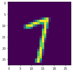

The corresponding label is:

CODE

example_label

CODE

Normalize the data set to improve the training speed, which means you need to know the mean and standard deviation:

CODE

mnist.data.float().mean() / 255, mnist.data.float().std() / 255

CODE

(tensor(0.1307), tensor(0.3081))

These are the values hard-coded in the transformations within the model. Ideally, you re-compute these based on the training data set to ensure you capture the correct values when the underlying data changes. This data set is static, though. Note that these values are always re-used (i.e. not re-computed) when predicting (or serving) to minimize training/serving skew. For this demonstration, it is fine to define these up front. Batch normalization would be an alternative that scales better with data sets of any size.

A Note on Batch Normalization
Batch normalization computes the mean and variance per batch of training data and per layer to rescale the batch's input values with the aid of two hyperparameters: β (shift) and γ (scale). It is typically applied before the activation function (as in the original paper), although there is no consensus on the matter and there may be valid reasons to apply it afterward. Batch normalization allows weights in later layers to be more robust against changes in input values of the earlier ones; while the input of later layers can obviously vary from step to step, the mean and variance will remain fairly constant. This is because you shuffle the training data set and each batch is therefore on average roughly representative of the entire data set. Batch normalization limits the distribution of weight values in the later layers of a neural network, and therefore provides a regularizing effect that decreases as the batch size increases.

At prediction time, batch normalization requires (fixed) values for the mean and variance to transform the data. The population statistics are the obvious choice, computed across batches from either moving averages or the exponentially weighted averages. It is often argued that you use these rather the equivalent values at inference time, because you may not receive batches to predict on; you cannot compute the mean and variance for individual examples. While that is certainly true in some cases (e.g. online predictions), the main reason is to avoid training/serving skew. Even with batches at inference, there may be significant correlation present (e.g. data from the same entity, such as a user, a session, a region, a product, a machine or assembly line, and so on). In these cases, the mean/variance of the prediction batch may not be representative of the population at large. Once scaled, these input values may well be near the population mean of zero with unit variance, even though in the overall population they would have been near the tails of the distribution.

CODE

# Clear variables that are no longer needed
del mnist, example, example_label

Before proceeding, we separate some of PyTorchJob parameters from the main code. The reason we do that is to ensure we can run the notebook in so-called headless mode with Papermill for custom parameters. This allows us to test the notebooks end-to-end automatically. If you check the cell tag of the next cell, you can see it is tagged as parameters. Feel free to ignore it!

CODE

EPOCHS = 5
GPUS = 1

Make the defined constants available as shell environment variables. They parameterize the PyTorchJob manifest below.

CODE

%env EPOCHS $EPOCHS
%env GPUS $GPUS

CODE

env: EPOCHS=5
env: GPUS=1

How to Train the Model in the Notebook

Since you ultimately want to train the model in a distributed fashion (potentially on GPUs), put all the code in a single cell. That way you can save the file and include it in a container image:

CODE

%%writefile $TRAINER_FILE
import argparse
import logging
import os

import torch
import torch.distributed as dist
import torch.nn as nn
import torch.nn.functional as F
import torch.optim as optim
import torch.utils.data
from torch.optim.lr_scheduler import StepLR
from torchvision import datasets, transforms

logging.getLogger().setLevel(logging.INFO)

# Number of processes participating in (distributed) job
# See: https://pytorch.org/docs/stable/distributed.html
WORLD_SIZE = int(os.environ.get("WORLD_SIZE", 1))


# Custom models must subclass toch.nn.Module and override `forward`
# See: https://pytorch.org/docs/stable/nn.html#torch.nn.Module
class Net(nn.Module):
    def __init__(self):
        super(Net, self).__init__()
        self.conv1 = nn.Conv2d(1, 32, 3, 1)
        self.conv2 = nn.Conv2d(32, 64, 3, 1)
        self.dropout1 = nn.Dropout2d(0.25)
        self.dropout2 = nn.Dropout2d(0.5)
        self.fc1 = nn.Linear(9216, 128)
        self.fc2 = nn.Linear(128, 10)

    def forward(self, x):
        x = self.conv1(x)
        x = F.relu(x)
        x = self.conv2(x)
        x = F.relu(x)
        x = F.max_pool2d(x, 2)
        x = self.dropout1(x)
        x = torch.flatten(x, 1)
        x = self.fc1(x)
        x = F.relu(x)
        x = self.dropout2(x)
        x = self.fc2(x)
        output = F.log_softmax(x, dim=1)
        return output


def should_distribute():
    return dist.is_available() and WORLD_SIZE > 1


def is_distributed():
    return dist.is_available() and dist.is_initialized()


def percentage(value):
    return "{: 5.1f}%".format(100.0 * value)


def train(args, model, device, train_loader, optimizer, epoch):
    model.train()
    for batch_idx, (data, target) in enumerate(train_loader):
        data, target = data.to(device), target.to(device)
        optimizer.zero_grad()
        output = model(data)
        loss = F.nll_loss(output, target)
        loss.backward()
        optimizer.step()
        if batch_idx % args.log_interval == 0:
            logging.info(
                f"Epoch: {epoch} ({percentage(batch_idx / len(train_loader))}) - Loss: {loss.item()}"
            )


def test(args, model, device, test_loader):
    model.eval()
    test_loss = 0
    correct = 0
    with torch.no_grad():
        for data, target in test_loader:
            data, target = data.to(device), target.to(device)
            output = model(data)
            test_loss += F.nll_loss(
                output, target, reduction="sum"
            ).item()  # sum batch losses
            pred = output.argmax(dim=1, keepdim=True)
            correct += pred.eq(target.view_as(pred)).sum().item()

    test_loss /= len(test_loader.dataset)

    logging.info(
        f"Test accuracy: {correct}/{len(test_loader.dataset)} ({percentage(correct / len(test_loader.dataset))})"
    )

    # Log metrics for Katib
    logging.info("loss={:.4f}".format(test_loss))
    logging.info("accuracy={:.4f}".format(float(correct) / len(test_loader.dataset)))


def main():
    parser = argparse.ArgumentParser(description="PyTorch MNIST Training Job")
    parser.add_argument(
        "--batch-size",
        type=int,
        default=64,
        metavar="N",
        help="Batch size for training (default: 64)",
    )
    parser.add_argument(
        "--test-batch-size",
        type=int,
        default=1000,
        metavar="N",
        help="Batch size for testing (default: 1000)",
    )
    parser.add_argument(
        "--epochs",
        type=int,
        default=5,
        metavar="N",
        help="Number of epochs to train",
    )
    parser.add_argument(
        "--lr",
        type=float,
        default=1.0,
        metavar="LR",
        help="Learning rate (default: 1.0)",
    )
    parser.add_argument(
        "--gamma",
        type=float,
        default=0.7,
        metavar="M",
        help="Learning rate's decay rate (default: 0.7)",
    )
    parser.add_argument(
        "--no-cuda",
        action="store_true",
        default=False,
        help="Disables CUDA (GPU) training",
    )
    parser.add_argument(
        "--seed", type=int, default=1, metavar="S", help="Random seed (default: 1)"
    )
    parser.add_argument(
        "--log-interval",
        type=int,
        default=10,
        metavar="N",
        help="Number of training batches between status log entries",
    )
    parser.add_argument(
        "--save-model",
        action="store_true",
        default=False,
        help="Whether to save the trained model",
    )

    if dist.is_available():
        parser.add_argument(
            "--backend",
            type=str,
            help="Distributed backend",
            choices=[dist.Backend.GLOO, dist.Backend.NCCL, dist.Backend.MPI],
            default=dist.Backend.GLOO,
        )

    args, _ = parser.parse_known_args()
    use_cuda = not args.no_cuda and torch.cuda.is_available()

    torch.manual_seed(args.seed)

    if should_distribute():
        logging.debug("Using distributed PyTorch with {} backend".format(args.backend))
        dist.init_process_group(backend=args.backend)

    kwargs = {"num_workers": 1, "pin_memory": True} if use_cuda else {}
    train_data = datasets.MNIST(
        "datasets",
        download=False,
        train=True,
        transform=transforms.Compose(
            [transforms.ToTensor(), transforms.Normalize((0.1307,), (0.3081,))]
        ),
    )

    # DistributedSampler partitions the training dataset among the worker processes
    train_sampler = (
        torch.utils.data.distributed.DistributedSampler(train_data)
        if should_distribute()
        else None
    )

    train_loader = torch.utils.data.DataLoader(
        train_data,
        batch_size=args.batch_size,
        sampler=train_sampler,
        shuffle=False,
        **kwargs,
    )

    test_loader = torch.utils.data.DataLoader(
        datasets.MNIST(
            "datasets",
            download=False,
            train=False,
            transform=transforms.Compose(
                [transforms.ToTensor(), transforms.Normalize((0.1307,), (0.3081,))]
            ),
        ),
        batch_size=args.test_batch_size,
        shuffle=True,
        **kwargs,
    )

    device = torch.device("cuda" if use_cuda else "cpu")
    model = Net().to(device)

    if is_distributed():
        if use_cuda:
            torch.cuda.set_device(torch.cuda.current_device())
        model = nn.parallel.DistributedDataParallel(model)

    # Check if GPUs are availible for CUDA-built image
    if int(os.getenv("GPUS",0)) > 0:
        if torch.cuda.get_device_name() is None:
            raise Exception(
                    f"Cannot find GPUs available using image with GPU support."
                )

    # See: https://pytorch.org/docs/stable/optim.html#torch.optim.Adadelta
    optimizer = optim.Adadelta(model.parameters(), lr=args.lr)

    # See: https://pytorch.org/docs/stable/optim.html#torch.optim.lr_scheduler.StepLR
    scheduler = StepLR(optimizer, step_size=1, gamma=args.gamma)
    for epoch in range(1, args.epochs + 1):
        train(args, model, device, train_loader, optimizer, epoch)
        test(args, model, device, test_loader)
        scheduler.step()

    if args.save_model:
        torch.save(model.state_dict(), "mnist_model.pt")


if __name__ == "__main__":
    main()

CODE

Writing mnist.py

That saves the file as defined by TRAINER_FILE but it does not run it.

The log entries for ‘Katib’ are to re-use the same file for hyperparameter tuning, which is done in a separate notebook. All you need to know for that is that Katib looks for key=value entries in the logs.

A Note on Activation Functions
A common choice for activation functions is a ReLU (Rectified Linear Unit). It is linear for non-negative values and zero for negative ones. The main benefits of ReLU as opposed to sigmoidal functions (e.g. logistic or `tanh`) are:

ReLU and its gradient are very cheap to compute;
Gradients are less likely to vanish, because for (non-)negative values its gradient is constant and therefore does not saturate, which for deep neural networks can accelerate convergence
ReLU has a regularizing effect, because it promotes sparse representations (i.e. some nodes' weights are zero);
Empirically it has been found to work well.

ReLU activation functions can cause neurons to 'die' because a large, negative (learned) bias value causes all inputs to be negative, which in turn leads to a zero output. The neuron has thus become incapable of discriminating different input values. So-called leaky ReLU activations functions address that issue; these functions are linear but non-zero for negative values, so that their gradients are small but non-zero. ELUs, or exponential linear units, are another solution to the problem of dying neurons.

A Note on CNNs
While it is not our intention to cover the basics of convolutional neural networks (CNNs), there are a few matters worth mentioning. Convolutional layers are spatial feature extractors for images. A series of convolutional kernels (of the same dimensions) is applied to the image to obtain different versions of the same base image (i.e. filters). These filters extract patterns hierarchically. In the first layer, filters typically capture dots, edges, corners, and so on. With each additional layer, these patterns become more complex and turn from basic geometric shapes into constituents of objects and entire objects. That is why often the number of filters increases with each additional convolutional layer: to extract more complex patterns.

Convolutional layers are often followed by a pooling layer to down-sample the input. This aids in lowering the computational burden as you increase the number of filters. A max pooling layer simply picks the largest value of pixels in a small (rectangular) neighbourhood of a single channel (e.g. RGB). This has the effect of making features locally translation-invariant, which is often desired: whether a feature of interest is on the left or right edge of a pooling window, which is also referred to as a kernel, is largely irrelevant to the problem of image classification. Note that this may not always be a desired characteristic and depends on the size of the pooling kernel. For instance, the precise location of tissue damage in living organisms or defects on manufactured products may be very significant indeed. Pooling kernels are generally chosen to be relatively small compared to the dimensions of the input, which means that local translation invariance is often desired.

Another common component of CNNs is a dropout layer. Dropout provides a mechanism for regularization that has proven successful in many applications. It is surprisingly simple: some nodes' weights (and biases) in a specific layer are set to zero at random, that is, arbitrary nodes are removed from the network during the training step. This causes the network to not rely on any single node (a.k.a. neuron) for a feature, as each node can be dropped at random. The network therefore has to learn redundant representations of features. This is important because of what is referred to as internal covariate shift (often mentioned in connection with batch normalization): the change of distributions of internal nodes' weights due to all other layers, which can cause nodes to stop learning (i.e. updating their weights). Thanks to dropout, layers become more robust to changes, although it also means it limits what can be learned (as always with regularization). Layers with a high risk of overfitting (e.g. layers with many units and lots of inputs) typically have a higher dropout rate.

A nice visual explanation of convolutional layers is available here. If you are curious what a CNN "sees" while training, you can have a look here.

Run the code from within the notebook to check that it is correct:

CODE

%run $TRAINER_FILE --epochs $EPOCHS --log-interval 128

CODE

INFO:root:Epoch: 1 (  0.0%) - Loss: 2.293032646179199
INFO:root:Epoch: 1 ( 13.6%) - Loss: 0.5257666110992432
INFO:root:Epoch: 1 ( 27.3%) - Loss: 0.08510863780975342
INFO:root:Epoch: 1 ( 40.9%) - Loss: 0.32805368304252625
INFO:root:Epoch: 1 ( 54.6%) - Loss: 0.3279671370983124
INFO:root:Epoch: 1 ( 68.2%) - Loss: 0.06365685909986496
INFO:root:Epoch: 1 ( 81.9%) - Loss: 0.29687821865081787
INFO:root:Epoch: 1 ( 95.5%) - Loss: 0.03434577211737633
INFO:root:Test accuracy: 9834/10000 ( 98.3%)
INFO:root:loss=0.0500
INFO:root:accuracy=0.9834
INFO:root:Epoch: 2 (  0.0%) - Loss: 0.08447802066802979
INFO:root:Epoch: 2 ( 13.6%) - Loss: 0.2620002329349518
INFO:root:Epoch: 2 ( 27.3%) - Loss: 0.10486980527639389
INFO:root:Epoch: 2 ( 40.9%) - Loss: 0.07522107660770416
INFO:root:Epoch: 2 ( 54.6%) - Loss: 0.044803790748119354
INFO:root:Epoch: 2 ( 68.2%) - Loss: 0.06450511515140533
INFO:root:Epoch: 2 ( 81.9%) - Loss: 0.25487586855888367
INFO:root:Epoch: 2 ( 95.5%) - Loss: 0.01875779777765274
INFO:root:Test accuracy: 9859/10000 ( 98.6%)
INFO:root:loss=0.0399
INFO:root:accuracy=0.9859
INFO:root:Epoch: 3 (  0.0%) - Loss: 0.029139619320631027
INFO:root:Epoch: 3 ( 13.6%) - Loss: 0.09397225826978683
INFO:root:Epoch: 3 ( 27.3%) - Loss: 0.11303514242172241
INFO:root:Epoch: 3 ( 40.9%) - Loss: 0.14118748903274536
INFO:root:Epoch: 3 ( 54.6%) - Loss: 0.05904180556535721
INFO:root:Epoch: 3 ( 68.2%) - Loss: 0.04524335265159607
INFO:root:Epoch: 3 ( 81.9%) - Loss: 0.27801263332366943
INFO:root:Epoch: 3 ( 95.5%) - Loss: 0.03176506236195564
INFO:root:Test accuracy: 9886/10000 ( 98.9%)
INFO:root:loss=0.0359
INFO:root:accuracy=0.9886
INFO:root:Epoch: 4 (  0.0%) - Loss: 0.07127423584461212
INFO:root:Epoch: 4 ( 13.6%) - Loss: 0.20250867307186127
INFO:root:Epoch: 4 ( 27.3%) - Loss: 0.0050563933327794075
INFO:root:Epoch: 4 ( 40.9%) - Loss: 0.14717304706573486
INFO:root:Epoch: 4 ( 54.6%) - Loss: 0.10025180876255035
INFO:root:Epoch: 4 ( 68.2%) - Loss: 0.13863351941108704
INFO:root:Epoch: 4 ( 81.9%) - Loss: 0.10420405864715576
INFO:root:Epoch: 4 ( 95.5%) - Loss: 0.004818277433514595
INFO:root:Test accuracy: 9887/10000 ( 98.9%)
INFO:root:loss=0.0329
INFO:root:accuracy=0.9887
INFO:root:Epoch: 5 (  0.0%) - Loss: 0.008954059332609177
INFO:root:Epoch: 5 ( 13.6%) - Loss: 0.19676166772842407
INFO:root:Epoch: 5 ( 27.3%) - Loss: 0.0015074732946231961
INFO:root:Epoch: 5 ( 40.9%) - Loss: 0.09220609813928604
INFO:root:Epoch: 5 ( 54.6%) - Loss: 0.015971817076206207
INFO:root:Epoch: 5 ( 68.2%) - Loss: 0.05801410600543022
INFO:root:Epoch: 5 ( 81.9%) - Loss: 0.07174661010503769
INFO:root:Epoch: 5 ( 95.5%) - Loss: 0.0020152931101620197
INFO:root:Test accuracy: 9909/10000 ( 99.1%)
INFO:root:loss=0.0306
INFO:root:accuracy=0.9909



<Figure size 432x288 with 0 Axes>

This trains the model in the notebook, but does not distribute it across nodes (a.k.a. pods) in the cluster. To that end, first create a Docker image with the code, push it to a registry (e.g. Docker Hub, Azure Container Registry, ECR, GCR), and then define the Kubernetes resource that uses the image.

How to Create a Docker Image with Kaptain SDK

Kaptain SDK allows you to build, push, and run containerized ML models without leaving Jupyter. To build and push Docker images from within a notebook, please check out the Build Docker Images with Kaptain SDK. All you need is the TRAINER_FILE and access to a container registry.

How to Create a Docker Image Manually

If you are comfortable with Docker (or prefer to use it as a part of your CI/CD setup), you can create a Dockerfile as follows. You do have to download the TRAINER_FILE contents to your local machine. The Kubernetes cluster does not have a Docker daemon available to build your image, so you must do it locally. It uses containerd to run workloads (only) instead.

The Dockerfile looks as follows:

CODE

FROM mesosphere/kubeflow:2.2.0-pytorch-1.11.0-gpu
ADD mnist.py /
ADD datasets /datasets

ENTRYPOINT ["python", "/mnist.py"]

If GPU support is not needed, you can leave off the -gpu suffix from the image. mnist.py is the trainer code you have to download to your local machine.

Then it is easy to push images to your container registry:

CODE

docker build -t <docker_image_name_with_tag> .
docker push <docker_image_name_with_tag>

The image is available as mesosphere/kubeflow:2.2.0-mnist-pytorch-1.11.0-gpu in case you want to skip it for now.

CODE

%env IMAGE mesosphere/kubeflow:2.2.0-mnist-pytorch-1.11.0-gpu

How to Create a Distributed`PyTorchJob`

For large training jobs, run the trainer in a distributed mode. Once the notebook server cluster can access the Docker image from the registry, you can launch a distributed PyTorch job.

The specification for a distributed PyTorchJob is defined using YAML:

CODE

%%bash
cat <<END > $KUBERNETES_FILE
apiVersion: "kubeflow.org/v1"
kind: "PyTorchJob"
metadata:
  name: "pytorchjob-mnist"
spec:
  pytorchReplicaSpecs:
    Master:
      replicas: 1
      restartPolicy: OnFailure
      template:
        metadata:
          annotations:
            sidecar.istio.io/inject: "false"
        spec:
          containers:
            - name: pytorch
              image: ${IMAGE}
              args:
                - --epochs
                - "${EPOCHS}"
                - --seed
                - "7"
                - --log-interval
                - "256"
                - --batch-size
                - "512"
              resources:
                limits:
                  cpu: 1
                  memory: "3G"
                  nvidia.com/gpu: ${GPUS}
    Worker:
      replicas: 2
      restartPolicy: OnFailure
      template:
        metadata:
          annotations:
            sidecar.istio.io/inject: "false"
        spec:
          containers:
            - name: pytorch
              image: ${IMAGE}
              args:
                - --epochs
                - "${EPOCHS}"
                - --seed
                - "7"
                - --log-interval
                - "256"
                - --batch-size
                - "512"
              resources:
                limits:
                  cpu: 1
                  memory: "3G"
                  nvidia.com/gpu: ${GPUS}
  runPolicy:
    ttlSecondsAfterFinished: 600
END

What this does is create one master and two worker pods. These can be adjusted via spec.pytorchReplicaSpecs.<type>.replicas with <type> either Master or Worker. The distributed sampler passes chunks of the training data set equally to the pods.

Custom training arguments can be passed to the container by means of the spec.containers.args. What is supported is visible in main() of mnist.py.

The container image specified (twice) is what is for the code shown above. Still, it’s best to change the image name listed under the comments of the specification to use an equivalent image in your own container registry, to ensure everything works as expected.

The job can run in parallel on CPUs or GPUs, provided these are available in your cluster. To switch to CPUs or define resource limits, please adjust spec.containers.resources as required.

To clean up finished PyTorchJob set spec.ttlSecondsAfterFinished. It may take extra ReconcilePeriod seconds for the cleanup, since reconcile gets called periodically. Defaults to infinite.

You can either execute the following commands on your local machine with kubectl or directly from the notebook. If you do run these locally, you cannot rely on cell magic, so you have to manually copy-paste the variables’ values wherever you see $SOME_VARIABLE. If you execute the following commands on your own machine (and not inside the notebook), you obviously do not need the cell magic %% lines either. In that case, you have to set the user namespace for all subsequent commands:

CODE

kubectl config set-context --current --namespace=<insert-namespace>

Please change the namespace to whatever has been set up by your administrator.

Deploy the distributed training job:

CODE

%%capture pytorch_output --no-stderr
%%sh
kubectl create -f "${KUBERNETES_FILE}"

CODE

%env PYTORCH_JOB {get_resource(pytorch_output)}

Check the status:

CODE

%%sh
kubectl describe $PYTORCH_JOB

The output looks like this:

CODE

Name:         pytorchjob-mnist
...
Kind:         PyTorchJob
...
Events:
  Type    Reason                   Age   From              Message
  ----    ------                   ----  ----              -------
  Normal  SuccessfulCreatePod      8s    pytorch-operator  Created pod: pytorchjob-mnist-master-0
  Normal  SuccessfulCreateService  8s    pytorch-operator  Created service: pytorchjob-mnist-master-0
  Normal  SuccessfulCreatePod      8s    pytorch-operator  Created pod: pytorchjob-mnist-worker-0
  Normal  SuccessfulCreatePod      8s    pytorch-operator  Created pod: pytorchjob-mnist-worker-1

You should now be able to see the pods created, matching the specified number of replicas.

CODE

%%sh
kubectl get pods -l job-name=pytorchjob-mnist

CODE

NAME                         READY   STATUS    RESTARTS   AGE
pytorchjob-mnist-master-0   1/1     Running   0          34s
pytorchjob-mnist-worker-0   1/1     Running   0          34s
pytorchjob-mnist-worker-1   1/1     Running   0          34s

The job name matches metadata.name from the YAML.

As per the specification, the training runs for 15 epochs. During that time, stream the logs from the Master pod to follow the progress:

CODE

%%sh
kubectl logs -f pytorchjob-mnist-master-0

CODE

Using distributed PyTorch with gloo backend
Epoch: 1 (  0.0%) - Loss: 2.3082287311553955
Epoch: 1 ( 81.8%) - Loss: 0.04400685429573059
Test accuracy: 9814/10000 ( 98.1%)
loss=0.0568
accuracy=0.9814
Epoch: 2 (  0.0%) - Loss: 0.12475904077291489
Epoch: 2 ( 81.8%) - Loss: 0.022593408823013306
Test accuracy: 9859/10000 ( 98.6%)
loss=0.0382
accuracy=0.9859
Epoch: 3 (  0.0%) - Loss: 0.10856910794973373
Epoch: 3 ( 81.8%) - Loss: 0.020849494263529778
Test accuracy: 9876/10000 ( 98.8%)
loss=0.0332
accuracy=0.9876
Epoch: 4 (  0.0%) - Loss: 0.09520195424556732
Epoch: 4 ( 81.8%) - Loss: 0.02882443554699421
Test accuracy: 9893/10000 ( 98.9%)
loss=0.0314
accuracy=0.9893
Epoch: 5 (  0.0%) - Loss: 0.09747796505689621
Epoch: 5 ( 81.8%) - Loss: 0.019643055275082588
Test accuracy: 9899/10000 ( 99.0%)
loss=0.0305
accuracy=0.9899
Epoch: 6 (  0.0%) - Loss: 0.02446436882019043
Epoch: 6 ( 81.8%) - Loss: 0.005831033922731876
Test accuracy: 9909/10000 ( 99.1%)
loss=0.0286
accuracy=0.9909
Epoch: 7 (  0.0%) - Loss: 0.024502133950591087
Epoch: 7 ( 81.8%) - Loss: 0.01055021770298481
Test accuracy: 9909/10000 ( 99.1%)
loss=0.0276
accuracy=0.9909
Epoch: 8 (  0.0%) - Loss: 0.02548063173890114
Epoch: 8 ( 81.8%) - Loss: 0.0008087620371952653
Test accuracy: 9907/10000 ( 99.1%)
loss=0.0272
accuracy=0.9907
Epoch: 9 (  0.0%) - Loss: 0.022815870121121407
Epoch: 9 ( 81.8%) - Loss: 0.003437922103330493
Test accuracy: 9908/10000 ( 99.1%)
loss=0.0272
accuracy=0.9908
Epoch: 10 (  0.0%) - Loss: 0.04595055431127548
Epoch: 10 ( 81.8%) - Loss: 0.00236672000028193
Test accuracy: 9908/10000 ( 99.1%)
loss=0.0267
accuracy=0.9908
Epoch: 11 (  0.0%) - Loss: 0.040099453181028366
Epoch: 11 ( 81.8%) - Loss: 0.003305426798760891
Test accuracy: 9912/10000 ( 99.1%)
loss=0.0267
accuracy=0.9912
Epoch: 12 (  0.0%) - Loss: 0.03731080889701843
Epoch: 12 ( 81.8%) - Loss: 0.006072529591619968
Test accuracy: 9909/10000 ( 99.1%)
loss=0.0270
accuracy=0.9909
Epoch: 13 (  0.0%) - Loss: 0.006752971094101667
Epoch: 13 ( 81.8%) - Loss: 0.0009820580016821623
Test accuracy: 9912/10000 ( 99.1%)
loss=0.0269
accuracy=0.9912
Epoch: 14 (  0.0%) - Loss: 0.019512642174959183
Epoch: 14 ( 81.8%) - Loss: 0.0012978784507140517
Test accuracy: 9912/10000 ( 99.1%)
loss=0.0268
accuracy=0.9912
Epoch: 15 (  0.0%) - Loss: 0.011409440077841282
Epoch: 15 ( 81.8%) - Loss: 0.0017151175998151302
Test accuracy: 9911/10000 ( 99.1%)
loss=0.0267
accuracy=0.9911

Note that it may take a while when the image has to be pulled from the registry. It usually takes a few minutes, depending on the arguments and resources of the cluster, for the status for all pods to be ‘Running’.

The setting spec.ttlSecondsAfterFinished will result in the cleanup of the created job:

CODE

%%sh
kubectl get pytorchjobs -w

CODE

NAME               STATE     AGE
pytorchjob-mnist   Created   0s
pytorchjob-mnist   Running   2s
pytorchjob-mnist   Running   2s
pytorchjob-mnist   Succeeded   70s
pytorchjob-mnist   Succeeded   70s
pytorchjob-mnist   Succeeded   11m

CODE

%%sh
kubectl get pytorchjob pytorchjob-mnist

To delete the job manually, execute:

CODE

%%sh
kubectl delete $PYTORCH_JOB

This tutorial includes code from the MinIO Project (“MinIO”), which is © 2014-2022 MinIO, Inc. MinIO is made available subject to the terms and conditions of the Apache Software Foundation, Apache License V2.0. The complete source code for the version of MinIO packaged with Kaptain 2.2.0 is available at this URL:

Minor Feature Release · minio/minio

For a full list of attributed 3rd party software, see http://d2iq.com/legal/3rd

Training MNIST with PyTorch

Introduction

What You Will Learn

What You Need

Prerequisites

How to Load and Inspect the Data

How to Train the Model in the Notebook

How to Create a Docker Image with Kaptain SDK

How to Create a Docker Image Manually

How to Create a DistributedPyTorchJob

How to Create a Distributed`PyTorchJob`