
MNIST with MXNet
NOTE: All tutorials in Jupyter Notebook format are available for download. You can either download them to a local computer and upload to the running Jupyter Notebook or run the following command from a Jupyter Notebook Terminal running in your Kaptain installation:
curl -L https://downloads.d2iq.com/kaptain/d2iq-tutorials-2.2.0.tar.gz | tar xzNOTE: These notebook tutorials have been built for and tested on D2iQ's Kaptain. Without the requisite Kubernetes operators and custom Docker images, these notebooks will likely not work.
Training MNIST with MXNet
Introduction
Recognizing handwritten digits based on the MNIST (Modified National Institute of Standards and Technology) data set is the “Hello, World” example of machine learning. Each (anti-aliased) black-and-white image represents a digit from 0 to 9 and fits in a 28×28 pixel bounding box. The problem of recognizing digits from handwriting is, for instance, important to the postal service when automatically reading zip codes from envelopes.
What You Will Learn
You will see how to use Apache MXNet to build a model with two convolutional layers and two fully connected layers to perform the multi-class classification of images provided.
What You Need
All you need is this notebook.
How to Load and Inspect the Data
Before proceeding, check you are using the correct notebook image, that is, MXNet is available:
%%sh
pip list | grep mxnetmxnet-cu102mkl 1.6.0Yes!
Import the necessary Python modules and load the data:
import mxnet as mx
import numpy as np

import gzip
import logging
import struct


logging.getLogger().setLevel(logging.INFO)


def get_mnist():
    """
    Utility method to load the MNIST dataset stored on disk.
    This is a modification of the original test_utils.get_mnist() function available in MXNet.

    Link:
    https://mxnet.apache.org/versions/1.6/api/python/docs/_modules/mxnet/test_utils.html#get_mnist
    """
    def read_data(label_url, image_url):
        with gzip.open(label_url) as flbl:
            struct.unpack(">II", flbl.read(8))
            label = np.frombuffer(flbl.read(), dtype=np.int8)
        with gzip.open(image_url, "rb") as fimg:
            _, _, rows, cols = struct.unpack(">IIII", fimg.read(16))
            image = np.frombuffer(fimg.read(), dtype=np.uint8).reshape(len(label), rows, cols)
            image = image.reshape(image.shape[0], 1, 28, 28).astype(np.float32)/255
        return label, image

    path = "datasets/mnist/"
    (train_lbl, train_img) = read_data(path+'train-labels-idx1-ubyte.gz', path+'train-images-idx3-ubyte.gz')
    (test_lbl, test_img) = read_data(path+'t10k-labels-idx1-ubyte.gz', path+'t10k-images-idx3-ubyte.gz')

    return {'train_data':train_img, 'train_label':train_lbl, 'test_data':test_img, 'test_label':test_lbl}


mnist = get_mnist()
For future reference, look at the available keys:
mnist.keys()dict_keys(['train_data', 'train_label', 'test_data', 'test_label'])How is the data structured? Grab an example and inspect the shape of the array:
example = mnist["train_data"][42]
example.shape(1, 28, 28)It has the shape (batch, height, width), because batch = 1 for a single example. For RGB images, the shape is (batch, height, width, channels) with channels = 3. What does the image itself look like?
import numpy as np

from matplotlib import pyplot as plt%matplotlib inline
plt.imshow(np.squeeze(example))
plt.show()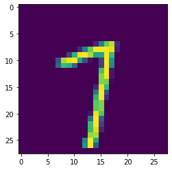
That could be both a 1 or a 7:
mnist["train_label"][42]7Just to be on the safe side, check the pixel values have already been scaled into the [0, 1] range:
flattened = example.flatten()
min(flattened), max(flattened)(0.0, 1.0)How to Train the Model
Please make use of the following convenience function to create a single convolutional layer with a certain activation function followed by a pre-defined max pooling layer. Since the model will have two such layers, it makes sense to package a single layer as a re-usable function.
A Note on Activation Functions
A common choice for activation functions is a ReLU (Rectified Linear Unit). It is linear for non-negative values and zero for negative ones. The main benefits of ReLU as opposed to sigmoidal functions (e.g. logistic or `tanh`) are:
ReLU and its gradient are very cheap to compute;
Gradients are less likely to vanish, because for (non-)negative values its gradient is constant and therefore does not saturate, which for deep neural networks can accelerate convergence
ReLU has a regularizing effect, because it promotes sparse representations (i.e. some nodes' weights are zero);
Empirically it has been found to work well.
ReLU activation functions can cause neurons to 'die' because a large, negative (learned) bias value causes all inputs to be negative, which in turn leads to a zero output. The neuron has thus become incapable of discriminating different input values. So-called leaky ReLU activations functions address that issue; these functions are linear but non-zero for negative values, so that their gradients are small but non-zero. ELUs, or exponential linear units, are another solution to the problem of dying neurons.
def conv_layer(input_layer, kernel, num_filters, activation):
    """
    Defines a CNN layer with `activation` function and 2D max pooling with a kernel and stride of (2, 2)

    :param layer: input layer (an MXNet symbol)
    :param kernel: 2D convolutional kernel
    :param filters: number of filters to use in convolution
    :param activation: activation function (e.g. "tanh" or "relu")
    :rtype: mxnet.symbol.symbol.Symbol
    """
    conv = mx.sym.Convolution(data=input_layer, kernel=kernel, num_filter=num_filters)
    act = mx.sym.Activation(data=conv, act_type=activation)
    pool = mx.sym.Pooling(data=act, pool_type="max", kernel=(2, 2), stride=(2, 2))
    return pool
A Note on CNNs
While it is not our intention to cover the basics of convolutional neural networks (CNNs), there are a few matters worth mentioning. Convolutional layers are spatial feature extractors for images. A series of convolutional kernels (of the same dimensions) is applied to the image to obtain different versions of the same base image (i.e. filters). These filters extract patterns hierarchically. In the first layer, filters typically capture dots, edges, corners, and so on. With each additional layer, these patterns become more complex and turn from basic geometric shapes into constituents of objects and entire objects. That is why often the number of filters increases with each additional convolutional layer: to extract more complex patterns.
Convolutional layers are often followed by a pooling layer to down-sample the input. This aids in lowering the computational burden as you increase the number of filters. A max pooling layer simply picks the largest value of pixels in a small (rectangular) neighbourhood of a single channel (e.g. RGB). This has the effect of making features locally translation-invariant, which is often desired: whether a feature of interest is on the left or right edge of a pooling window, which is also referred to as a kernel, is largely irrelevant to the problem of image classification. Note that this may not always be a desired characteristic and depends on the size of the pooling kernel. For instance, the precise location of tissue damage in living organisms or defects on manufactured products may be very significant indeed. Pooling kernels are generally chosen to be relatively small compared to the dimensions of the input, which means that local translation invariance is often desired.
Another common component of CNNs is a dropout layer. Dropout provides a mechanism for regularization that has proven successful in many applications. It is surprisingly simple: some nodes' weights (and biases) in a specific layer are set to zero at random, that is, arbitrary nodes are removed from the network during the training step. This causes the network to not rely on any single node (a.k.a. neuron) for a feature, as each node can be dropped at random. The network therefore has to learn redundant representations of features. This is important because of what is referred to as internal covariate shift (often mentioned in connection with batch normalization): the change of distributions of internal nodes' weights due to all other layers, which can cause nodes to stop learning (i.e. updating their weights). Thanks to dropout, layers become more robust to changes, although it also means it limits what can be learned (as always with regularization). Layers with a high risk of overfitting (e.g. layers with many units and lots of inputs) typically have a higher dropout rate.
A nice visual explanation of convolutional layers is available here. If you are curious what a CNN "sees" while training, you can have a look here.
With the following function, you create an ANN with two convolutional layers (as defined above), two fully connected layers with a different number of nodes, and an output layer with a softmax function. In each of the layers, choose the same activation function, although that is not needed and can easily be changed.
def ann(input_layer, kernels, filters, activation, hidden_units):
    """
    Defines a neural network with two convolutional layers and two dense layers.
    To train the model it needs to be wrapped in a module.

    :param input_layer: input layer (an MXNet symbol)
    :param kernels: a list of 2D convolutional kernels
    :param filters: a list of convolutional filters
    :param activation: the activation function for all layers (e.g. "tanh" or "relu")
    :param hidden_units: a list of hidden units for the dense layers
    :rtype: mxnet.symbol.symbol.Symbol
    """
    conv1 = conv_layer(
        input_layer=input_layer,
        kernel=kernels[0],
        num_filters=filters[0],
        activation=activation,
    )
    conv2 = conv_layer(
        input_layer=conv1,
        kernel=kernels[1],
        num_filters=filters[1],
        activation=activation,
    )

    flattened = mx.sym.flatten(data=conv2)

    fc1 = mx.sym.FullyConnected(data=flattened, num_hidden=hidden_units[0])
    fc1_out = mx.sym.Activation(data=fc1, act_type=activation)

    fc2 = mx.sym.FullyConnected(data=fc1_out, num_hidden=hidden_units[1])

    out = mx.sym.SoftmaxOutput(data=fc2, name="softmax")
    return out
Now it is time to define an execution context for the model training. If GPUs are available the model is trained on there. If not, it defaults to using CPUs.
Since you can use the context across training instances (e.g. if you want to see the effect of a different activation function), you can define it outside the main training loop:
context = mx.cpu()
if mx.context.num_gpus() > 0:
context = mx.gpu()epochs = 10
batch_size = 100import os
def train(
data,
context,
epochs,
batch_size,
learning_rate=0.1,
activation="tanh",
kernels=[(5, 5), (5, 5)],
filters=[20, 50],
hidden_units=[500, 10],
):
# Check if GPUs are availible for CUDA-built image
if os.path.exists("/usr/local/cuda"):
if mx.context.num_gpus() is 0:
raise Exception(
f"Cannot find GPUs available using image with GPU support."
)
# Create an iterator for the training data with a fixed `batch_size`
# Shuffle the data to ensure each batch is representative of the entire data set
# Note that you can also use `mxnet.test_utils.get_mnist_iterator`
train_iter = mx.io.NDArrayIter(
data["train_data"], data["train_label"], batch_size, shuffle=True
)
# Create an iterator for the test data with a fixed `batch_size`
# No need to shuffle the test data!
eval_iter = mx.io.NDArrayIter(data["test_data"], data["test_label"], batch_size)
# Define a symbolic (placeholder) variable
images = mx.sym.Variable("data")
# Create the artificial neural network based
net = ann(images, kernels, filters, activation, hidden_units)
# To be able to train (and evaluate) a model, you need the execution `context`,
# and you must wrap the (output) symbol `net` in a module.
model = mx.module.Module(symbol=net, context=context)
# Train using a stochastic gradient descent algorithm with respect to the test accuracy
model.fit(
train_iter,
eval_data=eval_iter,
optimizer="sgd",
optimizer_params={"learning_rate": learning_rate},
eval_metric="acc",
batch_end_callback=mx.callback.Speedometer(batch_size, 100),
num_epoch=epochs,
)
# Define another iterator and use the `score` method the `model` module
# to compute the accuracy.
# Note: You can see the accuracy on the training and test data set from the logs,
# but it is convenient to return it from the function, together with the model, so
# you can call `model.predict(...)` on it.
test_iter = mx.io.NDArrayIter(mnist["test_data"], mnist["test_label"], batch_size)
acc = mx.metric.Accuracy()
model.score(test_iter, acc)
return model, accInvoke it with the defaults (and the pre-defined parameters):
model, acc = train(mnist, context, epochs, batch_size)INFO:root:Epoch[0] Batch [0-100] Speed: 1353.96 samples/sec accuracy=0.114356
INFO:root:Epoch[0] Batch [100-200] Speed: 1438.84 samples/sec accuracy=0.113700
INFO:root:Epoch[0] Batch [200-300] Speed: 1464.64 samples/sec accuracy=0.112600
INFO:root:Epoch[0] Batch [300-400] Speed: 1523.29 samples/sec accuracy=0.109100
INFO:root:Epoch[0] Batch [400-500] Speed: 1467.58 samples/sec accuracy=0.113200
INFO:root:Epoch[0] Train-accuracy=0.112033
INFO:root:Epoch[0] Time cost=41.259
INFO:root:Epoch[0] Validation-accuracy=0.113500
INFO:root:Epoch[1] Batch [0-100] Speed: 1490.50 samples/sec accuracy=0.113069
INFO:root:Epoch[1] Batch [100-200] Speed: 1425.70 samples/sec accuracy=0.202600
INFO:root:Epoch[1] Batch [200-300] Speed: 1297.02 samples/sec accuracy=0.698700
INFO:root:Epoch[1] Batch [300-400] Speed: 1369.69 samples/sec accuracy=0.866400
INFO:root:Epoch[1] Batch [400-500] Speed: 1276.43 samples/sec accuracy=0.904900
INFO:root:Epoch[1] Train-accuracy=0.616617
INFO:root:Epoch[1] Time cost=44.176
INFO:root:Epoch[1] Validation-accuracy=0.931500
INFO:root:Epoch[2] Batch [0-100] Speed: 1347.37 samples/sec accuracy=0.935446
INFO:root:Epoch[2] Batch [100-200] Speed: 1332.14 samples/sec accuracy=0.949500
INFO:root:Epoch[2] Batch [200-300] Speed: 1287.23 samples/sec accuracy=0.955100
INFO:root:Epoch[2] Batch [300-400] Speed: 1245.89 samples/sec accuracy=0.956200
INFO:root:Epoch[2] Batch [400-500] Speed: 1289.72 samples/sec accuracy=0.961800
INFO:root:Epoch[2] Train-accuracy=0.953717
INFO:root:Epoch[2] Time cost=46.817
INFO:root:Epoch[2] Validation-accuracy=0.967500
INFO:root:Epoch[3] Batch [0-100] Speed: 1187.91 samples/sec accuracy=0.969604
INFO:root:Epoch[3] Batch [100-200] Speed: 1267.84 samples/sec accuracy=0.968600
INFO:root:Epoch[3] Batch [200-300] Speed: 1298.08 samples/sec accuracy=0.971600
INFO:root:Epoch[3] Batch [300-400] Speed: 1300.17 samples/sec accuracy=0.976300
INFO:root:Epoch[3] Batch [400-500] Speed: 1224.72 samples/sec accuracy=0.974500
INFO:root:Epoch[3] Train-accuracy=0.973083
INFO:root:Epoch[3] Time cost=47.699
INFO:root:Epoch[3] Validation-accuracy=0.977000
INFO:root:Epoch[4] Batch [0-100] Speed: 1233.89 samples/sec accuracy=0.975842
INFO:root:Epoch[4] Batch [100-200] Speed: 1286.16 samples/sec accuracy=0.981800
INFO:root:Epoch[4] Batch [200-300] Speed: 1167.10 samples/sec accuracy=0.979000
INFO:root:Epoch[4] Batch [300-400] Speed: 1246.25 samples/sec accuracy=0.979700
INFO:root:Epoch[4] Batch [400-500] Speed: 1202.52 samples/sec accuracy=0.982900
INFO:root:Epoch[4] Train-accuracy=0.980350
INFO:root:Epoch[4] Time cost=49.019
INFO:root:Epoch[4] Validation-accuracy=0.984200
INFO:root:Epoch[5] Batch [0-100] Speed: 1159.72 samples/sec accuracy=0.983366
INFO:root:Epoch[5] Batch [100-200] Speed: 1217.18 samples/sec accuracy=0.980900
INFO:root:Epoch[5] Batch [200-300] Speed: 1223.35 samples/sec accuracy=0.984400
INFO:root:Epoch[5] Batch [300-400] Speed: 1251.70 samples/sec accuracy=0.985000
INFO:root:Epoch[5] Batch [400-500] Speed: 1270.82 samples/sec accuracy=0.985400
INFO:root:Epoch[5] Train-accuracy=0.984067
INFO:root:Epoch[5] Time cost=48.736
INFO:root:Epoch[5] Validation-accuracy=0.984500
INFO:root:Epoch[6] Batch [0-100] Speed: 1225.29 samples/sec accuracy=0.986139
INFO:root:Epoch[6] Batch [100-200] Speed: 1180.46 samples/sec accuracy=0.986300
INFO:root:Epoch[6] Batch [200-300] Speed: 1272.58 samples/sec accuracy=0.986600
INFO:root:Epoch[6] Batch [300-400] Speed: 1276.39 samples/sec accuracy=0.985300
INFO:root:Epoch[6] Batch [400-500] Speed: 1295.95 samples/sec accuracy=0.989000
INFO:root:Epoch[6] Train-accuracy=0.986550
INFO:root:Epoch[6] Time cost=48.073
INFO:root:Epoch[6] Validation-accuracy=0.987700
INFO:root:Epoch[7] Batch [0-100] Speed: 1213.19 samples/sec accuracy=0.986931
INFO:root:Epoch[7] Batch [100-200] Speed: 1157.00 samples/sec accuracy=0.987300
INFO:root:Epoch[7] Batch [200-300] Speed: 1182.32 samples/sec accuracy=0.988800
INFO:root:Epoch[7] Batch [300-400] Speed: 1250.13 samples/sec accuracy=0.989800
INFO:root:Epoch[7] Batch [400-500] Speed: 1226.76 samples/sec accuracy=0.989100
INFO:root:Epoch[7] Train-accuracy=0.988350
INFO:root:Epoch[7] Time cost=49.748
INFO:root:Epoch[7] Validation-accuracy=0.987400
INFO:root:Epoch[8] Batch [0-100] Speed: 1262.47 samples/sec accuracy=0.990990
INFO:root:Epoch[8] Batch [100-200] Speed: 1199.14 samples/sec accuracy=0.989800
INFO:root:Epoch[8] Batch [200-300] Speed: 1193.96 samples/sec accuracy=0.990500
INFO:root:Epoch[8] Batch [300-400] Speed: 1087.18 samples/sec accuracy=0.988200
INFO:root:Epoch[8] Batch [400-500] Speed: 1154.58 samples/sec accuracy=0.989800
INFO:root:Epoch[8] Train-accuracy=0.989850
INFO:root:Epoch[8] Time cost=50.834
INFO:root:Epoch[8] Validation-accuracy=0.988700
INFO:root:Epoch[9] Batch [0-100] Speed: 1179.14 samples/sec accuracy=0.990297
INFO:root:Epoch[9] Batch [100-200] Speed: 1226.71 samples/sec accuracy=0.990800
INFO:root:Epoch[9] Batch [200-300] Speed: 1208.98 samples/sec accuracy=0.989800
INFO:root:Epoch[9] Batch [300-400] Speed: 1272.81 samples/sec accuracy=0.991500
INFO:root:Epoch[9] Batch [400-500] Speed: 1292.01 samples/sec accuracy=0.989900
INFO:root:Epoch[9] Train-accuracy=0.990800
INFO:root:Epoch[9] Time cost=48.257
INFO:root:Epoch[9] Validation-accuracy=0.987700A Note on Accuracy
You can see from the logs that the accuracy on both training and test data are relatively close. A training accuracy that is significantly higher than the test accuracy is an indication of a model that overfits: it picks up on noise rather than the signal that is present in the data. This model, therefore, does a decent job of classifying digits in images.
Because you wrapped the training process in a function, you can easily see the impact of a different activation function:
model_relu, acc_relu = train(mnist, context, epochs, batch_size, activation="relu")INFO:root:Epoch[0] Batch [0-100] Speed: 1693.27 samples/sec accuracy=0.111089
INFO:root:Epoch[0] Batch [100-200] Speed: 1739.83 samples/sec accuracy=0.118500
INFO:root:Epoch[0] Batch [200-300] Speed: 1768.59 samples/sec accuracy=0.105400
INFO:root:Epoch[0] Batch [300-400] Speed: 1870.50 samples/sec accuracy=0.112700
INFO:root:Epoch[0] Batch [400-500] Speed: 1777.87 samples/sec accuracy=0.111900
INFO:root:Epoch[0] Train-accuracy=0.112017
INFO:root:Epoch[0] Time cost=33.978
INFO:root:Epoch[0] Validation-accuracy=0.113500
INFO:root:Epoch[1] Batch [0-100] Speed: 1813.15 samples/sec accuracy=0.117228
INFO:root:Epoch[1] Batch [100-200] Speed: 1764.89 samples/sec accuracy=0.107800
INFO:root:Epoch[1] Batch [200-300] Speed: 1798.58 samples/sec accuracy=0.113700
INFO:root:Epoch[1] Batch [300-400] Speed: 1880.55 samples/sec accuracy=0.235100
INFO:root:Epoch[1] Batch [400-500] Speed: 1829.45 samples/sec accuracy=0.713800
INFO:root:Epoch[1] Train-accuracy=0.360967
INFO:root:Epoch[1] Time cost=32.823
INFO:root:Epoch[1] Validation-accuracy=0.935800
INFO:root:Epoch[2] Batch [0-100] Speed: 1876.07 samples/sec accuracy=0.928416
INFO:root:Epoch[2] Batch [100-200] Speed: 1837.19 samples/sec accuracy=0.942200
INFO:root:Epoch[2] Batch [200-300] Speed: 1892.24 samples/sec accuracy=0.952900
INFO:root:Epoch[2] Batch [300-400] Speed: 1895.88 samples/sec accuracy=0.961800
INFO:root:Epoch[2] Batch [400-500] Speed: 1943.46 samples/sec accuracy=0.962000
INFO:root:Epoch[2] Train-accuracy=0.952467
INFO:root:Epoch[2] Time cost=31.772
INFO:root:Epoch[2] Validation-accuracy=0.970900
INFO:root:Epoch[3] Batch [0-100] Speed: 1884.76 samples/sec accuracy=0.965248
INFO:root:Epoch[3] Batch [100-200] Speed: 1930.55 samples/sec accuracy=0.974600
INFO:root:Epoch[3] Batch [200-300] Speed: 1932.68 samples/sec accuracy=0.973000
INFO:root:Epoch[3] Batch [300-400] Speed: 1919.08 samples/sec accuracy=0.975500
INFO:root:Epoch[3] Batch [400-500] Speed: 1875.23 samples/sec accuracy=0.977300
INFO:root:Epoch[3] Train-accuracy=0.973900
INFO:root:Epoch[3] Time cost=31.617
INFO:root:Epoch[3] Validation-accuracy=0.981600
INFO:root:Epoch[4] Batch [0-100] Speed: 1882.73 samples/sec accuracy=0.976832
INFO:root:Epoch[4] Batch [100-200] Speed: 1879.33 samples/sec accuracy=0.978900
INFO:root:Epoch[4] Batch [200-300] Speed: 1696.34 samples/sec accuracy=0.981700
INFO:root:Epoch[4] Batch [300-400] Speed: 1771.81 samples/sec accuracy=0.982200
INFO:root:Epoch[4] Batch [400-500] Speed: 1779.80 samples/sec accuracy=0.982500
INFO:root:Epoch[4] Train-accuracy=0.980533
INFO:root:Epoch[4] Time cost=33.584
INFO:root:Epoch[4] Validation-accuracy=0.983500
INFO:root:Epoch[5] Batch [0-100] Speed: 1888.09 samples/sec accuracy=0.984653
INFO:root:Epoch[5] Batch [100-200] Speed: 1830.69 samples/sec accuracy=0.987400
INFO:root:Epoch[5] Batch [200-300] Speed: 1752.42 samples/sec accuracy=0.985500
INFO:root:Epoch[5] Batch [300-400] Speed: 1716.19 samples/sec accuracy=0.983000
INFO:root:Epoch[5] Batch [400-500] Speed: 1728.71 samples/sec accuracy=0.985200
INFO:root:Epoch[5] Train-accuracy=0.985150
INFO:root:Epoch[5] Time cost=33.577
INFO:root:Epoch[5] Validation-accuracy=0.983600
INFO:root:Epoch[6] Batch [0-100] Speed: 1829.37 samples/sec accuracy=0.988119
INFO:root:Epoch[6] Batch [100-200] Speed: 1879.84 samples/sec accuracy=0.988000
INFO:root:Epoch[6] Batch [200-300] Speed: 1866.12 samples/sec accuracy=0.988600
INFO:root:Epoch[6] Batch [300-400] Speed: 1901.34 samples/sec accuracy=0.988500
INFO:root:Epoch[6] Batch [400-500] Speed: 1850.14 samples/sec accuracy=0.986400
INFO:root:Epoch[6] Train-accuracy=0.988083
INFO:root:Epoch[6] Time cost=32.148
INFO:root:Epoch[6] Validation-accuracy=0.985400
INFO:root:Epoch[7] Batch [0-100] Speed: 1834.51 samples/sec accuracy=0.990891
INFO:root:Epoch[7] Batch [100-200] Speed: 1873.71 samples/sec accuracy=0.989500
INFO:root:Epoch[7] Batch [200-300] Speed: 1878.99 samples/sec accuracy=0.989000
INFO:root:Epoch[7] Batch [300-400] Speed: 1879.32 samples/sec accuracy=0.989200
INFO:root:Epoch[7] Batch [400-500] Speed: 1815.73 samples/sec accuracy=0.989600
INFO:root:Epoch[7] Train-accuracy=0.989600
INFO:root:Epoch[7] Time cost=32.270
INFO:root:Epoch[7] Validation-accuracy=0.987400
INFO:root:Epoch[8] Batch [0-100] Speed: 1732.95 samples/sec accuracy=0.991188
INFO:root:Epoch[8] Batch [100-200] Speed: 1635.98 samples/sec accuracy=0.988900
INFO:root:Epoch[8] Batch [200-300] Speed: 1799.76 samples/sec accuracy=0.992300
INFO:root:Epoch[8] Batch [300-400] Speed: 1736.55 samples/sec accuracy=0.992600
INFO:root:Epoch[8] Batch [400-500] Speed: 1825.21 samples/sec accuracy=0.990400
INFO:root:Epoch[8] Train-accuracy=0.991017
INFO:root:Epoch[8] Time cost=34.618
INFO:root:Epoch[8] Validation-accuracy=0.987800
INFO:root:Epoch[9] Batch [0-100] Speed: 1749.84 samples/sec accuracy=0.991881
INFO:root:Epoch[9] Batch [100-200] Speed: 1813.36 samples/sec accuracy=0.991900
INFO:root:Epoch[9] Batch [200-300] Speed: 1832.93 samples/sec accuracy=0.992500
INFO:root:Epoch[9] Batch [300-400] Speed: 1561.59 samples/sec accuracy=0.994700
INFO:root:Epoch[9] Batch [400-500] Speed: 1848.26 samples/sec accuracy=0.992400
INFO:root:Epoch[9] Train-accuracy=0.992583
INFO:root:Epoch[9] Time cost=34.517
INFO:root:Epoch[9] Validation-accuracy=0.987800print(f"Accuracy: {acc} (tanh) vs {acc_relu} (ReLU)")Accuracy: EvalMetric: {'accuracy': 0.9877} (tanh) vs EvalMetric: {'accuracy': 0.9878} (ReLU)This is just a simple example of fiddling with hyperparameters. If you wanted to tune hyperparameters (with Katib) automatically, you could simply pass these hyperparameters as arguments to the container that contains a script with all necessary imports and functions to run the train-and-evaluate process.
How to Predict with a Trained Model
Batch predictions based on a trained model are easy:
def test_iter(data=mnist, batch_size=100):
    return mx.io.NDArrayIter(data["test_data"], None, batch_size=batch_size)


prob = model.predict(test_iter())
prob_relu = model_relu.predict(test_iter())
If you pick a random example, you can see the probabilities per category (i.e. digit):
prob[24], prob_relu[24](
[3.88936355e-10 5.50869439e-09 1.38218335e-08 1.33717464e-11
9.99999046e-01 1.08974885e-09 3.25030669e-07 8.28973228e-08
1.59384072e-07 3.14834097e-07]
<NDArray 10 @cpu(0)>,
[6.4347176e-08 7.3004806e-08 3.4015596e-08 5.8196594e-09 9.9998724e-01
1.2476704e-07 1.9580840e-07 3.0599865e-06 1.2806310e-08 9.1640350e-06]
<NDArray 10 @cpu(0)>)The highest probability is observed for the fourth index (i.e. the digit ‘4’):
np.argmax(prob[24]), np.argmax(prob_relu[24])(
[4.]
<NDArray 1 @cpu(0)>,
[4.]
<NDArray 1 @cpu(0)>)Since you did not shuffle data for the iterator test_iter that was used to generate probabilities, you can use the same index to obtain the label to verify that the model predicts the digit correctly:
mnist["test_label"][24]4This tutorial includes code from the MinIO Project (“MinIO”), which is © 2014-2022 MinIO, Inc. MinIO is made available subject to the terms and conditions of the Apache Software Foundation, Apache License V2.0. The complete source code for the version of MinIO packaged with Kaptain 2.2.0 is available at this URL:
For a full list of attributed 3rd party software, see http://d2iq.com/legal/3rd